How to train a segmentation model for car parts

In this blog post, we will discuss how to train a segmentation model for car parts using the keras UNET model.
We will provide a complete example of how to use the trained model to identify cars components.
What do we need:
The dataset:
We are using de car parts dataset that you can find here: https://github.com/dsmlr/Car-Parts-Segmentation
The Model framework:
We are using the Segmentation models library which is a python library with Neural Networks for Image Segmentation based on Keras
The COCO API:
This is a package for help us to process the images properly create the annotations
Let’s install all of them:
!pip -qq install -U  segmentation-models

!pip -qq install git+https://github.com/philferriere/cocoapi.git#subdirectory=PythonAPI

!git clone https://github.com/dsmlr/Car-Parts-Segmentation.git
Now we need to create the folder were the annotations and image will be placed:
!mkdir /content/Car-Parts-Segmentation/trainingset/annotations/

!mkdir /content/Car-Parts-Segmentation/valset

!mkdir /content/Car-Parts-Segmentation/valset/JPEGImages

!mkdir /content/Car-Parts-Segmentation/valset/annotations

!mkdir /content/Car-Parts-Segmentation/testset/annotations
Let’s explore the images of the dataset:
I = cv2.imread( '/content/Car-Parts-Segmentation/trainingset/JPEGImages/train1.jpg' ) I.shape#The output:#(512, 512, 3)
All the images in the dataset are 512×512 RGB (means that our model must math that input size and we need to process any new images to match that dimensions)
Let’s plot it:
plt.imshow(I)

The annotations:
With the images, the cars-parts dataset have a file called “annotations.json” which is a file that contains every segment present in all the images of the data.
This dataset contains annotations for 19 car’s segments:
We need to transforms these annotations segment into images to train our segmentation model.
To properly process the annotations file we use the COCO API helper:
from pycocotools.coco import COCO

coco=COCO('/content/Car-Parts-Segmentation/trainingset/annotations.json')

print(f"The categories Ids: {coco.getCatIds()}")
The output:
The categories Ids: [1, 2, 3, 4, 5, 6, 7, 8, 9, 10, 11, 12, 13, 14, 15, 16, 17, 18, 19]
You can see that the COCO API is reading properly the annotations and there are 19 annotations as we said earlier.
Now we need, using the anotations file, create a segment image, it means for each image on the dataset create a new image with all pixel equal zero, EXCEPT the pixels where is a segment, that’s will be our segment image what the model is going to learn to predict.
Example:
Input Image: this is the input image for the model

Segment Image, this is what the model is going to predict:

Why the segment image is almost all black? that’s because the pixels values are not zero just in the segment labeled and its values is the categoryId value which is going from 1-18, close to zero (remember the pixel value from a given images is 0-255)
For each image present we need a segment image, so we use this function to create all the segment images:
anno_dir = '/content/Car-Parts-Segmentation/trainingset/annotations/'
img_dir = '/content/Car-Parts-Segmentation/trainingset/JPEGImages/'

def create_label_img(anno_dir, img_dir, coco):
  catIds = coco.getCatIds()
  for im_id in coco.getImgIds():
    img = coco.loadImgs(im_id)[0]
    annIds = coco.getAnnIds(imgIds=img['id'], catIds=catIds, iscrowd=None)
    I = cv2.imread( img_dir + img['file_name'] )
    anns = coco.loadAnns(annIds)
    if isinstance(I, np.ndarray):
      anns_img = np.zeros((I.shape[0], I.shape[1]))
      for i,ann in enumerate(anns):
          if ann['category_id'] != 0:
            anns_img[(coco.annToMask(ann) != 0)] = ann['category_id'] -1
      f_name = img['file_name'].split(".")[0] +'.png'
      cv2.imwrite(anno_dir+ f_name ,anns_img )


create_label_img(anno_dir, img_dir, coco)
The output is the annotation directory with all the new segment images.
Now we need to make the same with the test images, and because the data set does not have a validation images, we are going to split the test images into test al folder 50:50
source_dir = '/content/Car-Parts-Segmentation/testset/JPEGImages/'
target_dir = '/content/Car-Parts-Segmentation/valset/JPEGImages/'

if len(os.listdir(target_dir )) != 50:
  file_names = os.listdir(source_dir)

  random.shuffle(file_names)

  for file_name in file_names[:50]:
    shutil.move(os.path.join(source_dir, file_name), target_dir)
anno_dir_v = '/content/Car-Parts-Segmentation/valset/annotations/'
img_dir_v = '/content/Car-Parts-Segmentation/valset/JPEGImages/'
coco_v=COCO('/content/Car-Parts-Segmentation/testset/annotations.json')

if len(os.listdir(y_valid_dir))!=50:
  create_label_img(anno_dir_v, img_dir_v, coco_v)
When finish let’s check how many images we got:
print('the number of image/label in the train: ',len(os.listdir(x_train_dir)))
print('the number of image/label in the validation: ',len(os.listdir(x_valid_dir)))
The output:
the number of image/label in the train: 400
the number of image/label in the validation: 50
Now let’s explore the data we have
# Lets look at data we have
dataset = Dataset(x_train_dir, y_train_dir, classes=c)

image, mask = dataset[37] # get some sample
visualize(
    image=image,
    background_mask=mask[..., 0].squeeze(),
    hood_mask=mask[..., 13].squeeze(),
    wheel_mask=mask[..., 18].squeeze(),
)
We create a Dataset class for load the dataset, the full code implementation is on github, is just a helper class to handle the data loading
The output showing the background, the hood and the wheel segment for a random images is:

The data loading seems good.
Because the dataset is small, we need a way to increase the dataset that is made by applying data augmentation, that is apply random variations to the images to create “a new image”
for this we uses the library albumentations we allow us apply variation like rotation, translation, padding, sharpen, gaussian noise etc.
The output showing the background, the hood and the wheel segment for a random images after apply augmentation is:

you can seen some random image distortions.
The augmentation technique allow us to achieve better generalization
The Model Part:
We are using the U-Net architecture, which is a widely used deep learning network that can be used for image segmentation, it essentially use a arrange of layers that can be understanding as encoder-decoder in U-form.
There a re extensive resource to learn more deeply about u-net,
In this blog we are using a pre-trained encoder called “resnet18” and keras as our deep learning framework.
Let’s do it:
import segmentation_models as sm
sm.set_framework('tf.keras')

sm.framework()

BACKBONE = 'resnet18' #Here we select the encoder
BATCH_SIZE = 4
CLASSES = c
LR = 0.0002
EPOCHS = 40

preprocess_input = sm.get_preprocessing(BACKBONE)

# define network parameters
n_classes = 1 if len(CLASSES) == 1 else (len(CLASSES))  # case for binary and multiclass segmentation
activation = 'sigmoid' if n_classes == 1 else 'softmax'

#create model
model = sm.Unet(BACKBONE, classes=n_classes, activation=activation)

# define optomizer
optim = tf.keras.optimizers.Adam(LR)
The output:
The loss function:
Loss function for image segmentation tasks is based on two loss the Dice loss and the focal loss.
The Dice loss is based on the Dice coefficient, which is essentially a measure of overlap between two samples. This measure ranges from 0 to 1 where a Dice coefficient of 1 denotes perfect and complete overlap.
The dice loss can be defined as:

where |A∩B||A∩B| represents the common segments between sets A and B, in this case A could be the real segments and B the predicted one.
And the focal loss:
This is similar to the cross entropy loss with an extra term that force to focus on misclassified ones, you can see more here.
Focal loss can be defined as:

where Pt represents the probability and γ (Gamma) is the focusing parameter
We are using the dice loss plus focal loss as our loss function.
In the code:
# Segmentation models losses can be combined together by '+' and scaled by integer or float factor
# set class weights for dice_loss
dice_loss = sm.losses.DiceLoss(class_weights=np.array([0.5, 1,1,2,1,2,1,1.5,1.2,2,1,2,1,1.5,1,1,1,1,2]))

focal_loss = sm.losses.BinaryFocalLoss() if n_classes == 1 else sm.losses.CategoricalFocalLoss()

total_loss = dice_loss + (1 * focal_loss)

# actulally total_loss can be imported directly from library, above example just show you how to manipulate with losses
When defining the dice loss you can assigns weights to the classes in order to give more importance to a particular class, for example we assign the smallest value (0.5) to the background segment because we don’t want that the model learn too much about the background and forget about car lights for example.
Metrics:
We are using the Intersect over Union (IoU) and the F1 Score as our metrics.
The IoU allows us to evaluate how similar our predicted segment is to the ground truth segment.
Iou is defined as:

Graphically:

The closest is IoU to 1, the better the model is.
Finally the F1 Score is the metric that combines the precision and recall of a classifier into a single metric by taking their harmonic mean, check more here.
in the code:
metrics = [sm.metrics.IOUScore(threshold=0.5), sm.metrics.FScore(threshold=0.5)]

# compile keras model with defined optimizer, loss and metrics
model.compile(optim, total_loss, metrics)
Training:
Now that we have the data, the annotation masks, the loss and metrics is time to train the model
We create the Keras data loader, it help us to Load data from dataset and form batches.
# Dataset for train images
train_dataset = Dataset(
    x_train_dir,
    y_train_dir,
    classes=CLASSES,
    augmentation=get_training_augmentation(),
    preprocessing=get_preprocessing(preprocess_input),
)

# Dataset for validation images
valid_dataset = Dataset(
    x_valid_dir,
    y_valid_dir,
    classes=CLASSES,
    augmentation=get_validation_augmentation(),
    preprocessing=get_preprocessing(preprocess_input),
)

train_dataloader = Dataloder(train_dataset, batch_size=BATCH_SIZE, shuffle=True)
valid_dataloader = Dataloder(valid_dataset, batch_size=1, shuffle=False)
Define callbacks for learning rate scheduling and best checkpoints saving:
callbacks = [
    keras.callbacks.ModelCheckpoint('./best_model.h5', save_weights_only=True, save_best_only=True, mode='min'),
    keras.callbacks.ReduceLROnPlateau(),
]
And train the model:
# train model
history = model.fit(
    train_dataloader,
    steps_per_epoch=len(train_dataloader),
    epochs=EPOCHS,
    callbacks=callbacks,
    validation_data=valid_dataloader,
    validation_steps=len(valid_dataloader),
)
After 40 epoch we got the following results:


When seeing the loss plot seems like our model is overfitting, also the gap between the losses could mean that the training dataset has too few examples as compared to the validation dataset, we need more data or add more augmentations to our model.
However also seems like is have good validation metrics, let’s explore visually the predictions
Results:
Now that we have the model trained let’s check how the results are:
First, check the metrics on the 50-images of the test dataset:
scores = model.evaluate_generator(test_dataloader)

print("Loss: {:.5}".format(scores[0]))
for metric, value in zip(metrics, scores[1:]):
    print("mean {}: {:.5}".format(metric.__name__, value))
It print:
Loss: 0.5671
mean iou_score: 0.74382
mean f1-score: 0.77697
Not bad, let explore some images, by selecting 3 random images from the test set and visualize the predictions:
n = 3
ids = np.random.choice(np.arange(len(test_dataset)), size=n)

for i in ids:

    image, gt_mask = test_dataset[i]
    # image = np.expand_dims(I['image'], axis=0)
    image = np.expand_dims(image, axis=0)
    pr_mask = model.predict(image).squeeze()

    gt_mask_gray = np.zeros((gt_mask.shape[0],gt_mask.shape[1]))

    for ii in range(gt_mask.shape[2]):
        gt_mask_gray = gt_mask_gray + 1/gt_mask.shape[2]*ii*gt_mask[:,:,ii]

    pr_mask_gray = np.zeros((pr_mask.shape[0],pr_mask.shape[1]))
    for ii in range(pr_mask.shape[2]):
        pr_mask_gray = pr_mask_gray + 1/pr_mask.shape[2]*ii*pr_mask[:,:,ii]

    visualize(
        image=denormalize(image.squeeze()),
        gt_mask=gt_mask_gray,
        pr_mask=pr_mask_gray,
    )


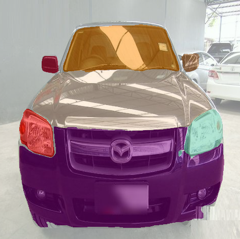
It seems the model is able to recognize the car’s segments properly, you can see the original image, the true segments (Gt Mask) and the predicted segments (Pr Mask)
Maybe labeling more data or change the backbone model could improve this predictions. For example with need to collect more images from internet, labeled them and create a annotation.json with the new images in order to add to the train dataset.
Remember all the code along with the requirements.txt can be found on my github repo.
If you like this post please consider subscribe and follow me on twitter.
Try the live model:
I created this app in order you can check the model in action with your own image: